bmripper
Artificial Intelligence Project
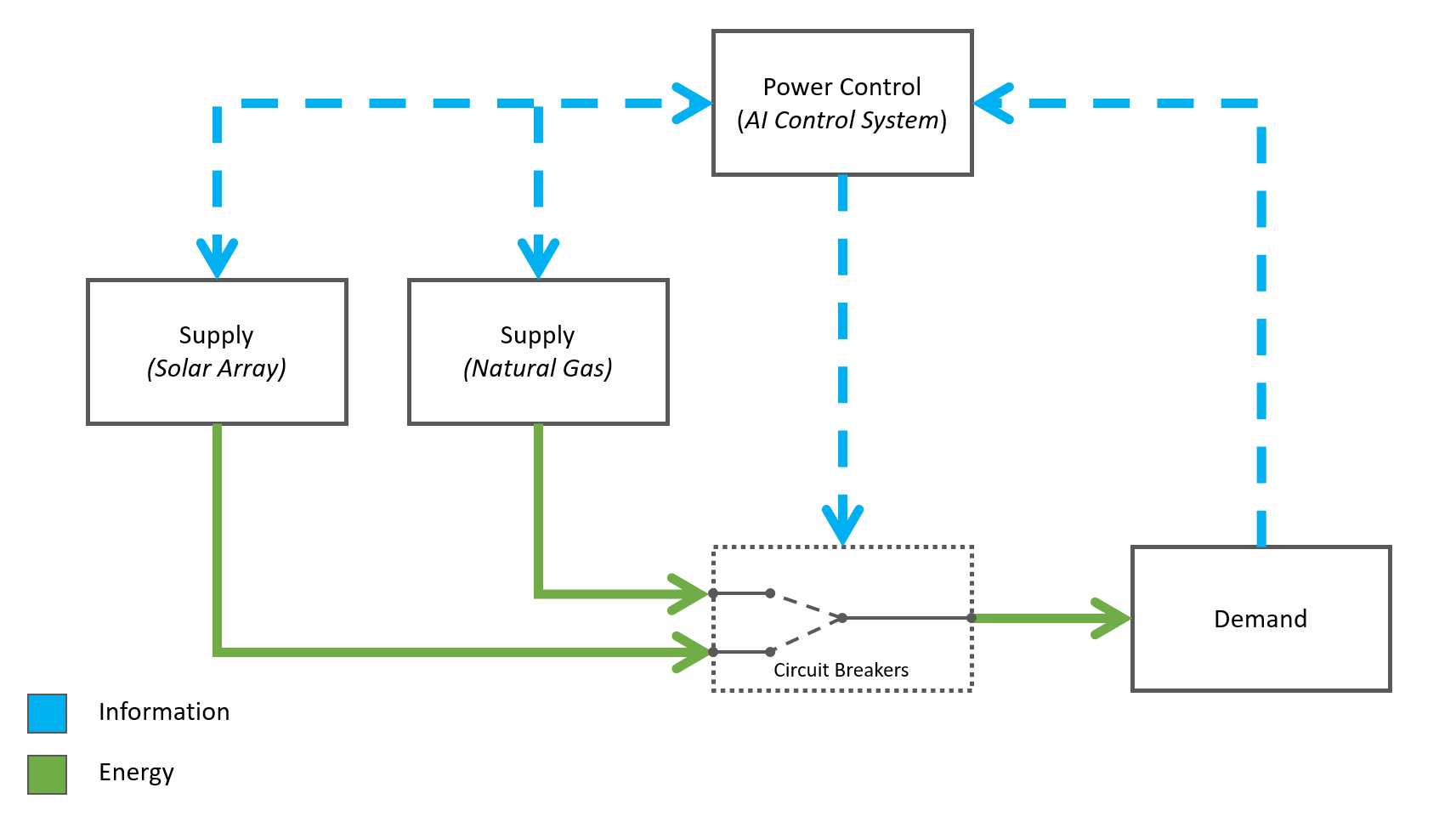
The project demonstrates my work in Artifical Intelligence (AI), specially Reinforcement Learning. I am attempting to create a control system for distributed energy resources (DERs) using AI. The project was my initial attempt at a simple model: learn the optimal operator action plan for a power plant with solar panels and a natural gas turbine (i.e., at which hours should I run the natural gas turbine). I created a simulator in Excel first, then recreated the simulator in Python. The script uses reinforcement learning to find the optimal path (operator action plan) for a 24 hour period. While the system is simple, it was an effective test to determine the feasibility of the control system idea.
Big thanks to Mic (2016) for providing a major part of the model’s navigation code in the state-action space, Getting AI smarter with Q-learning: a simple first step in Python!
| header | value |
|---|---|
| Program: | html file |
| Author: | Ripperger, Brent |
| Date Created: | 21 May 2022 |
Problem Setup
Environment
| source | variable | qty | UoM |
|---|---|---|---|
| Solar | Cloud Coverage | 0.3 | prop. of area |
| Solar | St.D Cloud Coverage | 0.1 | prop. of area |
| Solar | Irradiance | 7 | kJ/m2 |
| Solar | Area | 100 | m2 |
| NG | Power | 70 | kW |
| NG | Up-Time | 0.95 | % runtime |
Rules
| variable | qty | UoM |
|---|---|---|
| Goal | 50 | kWh |
| Reward Function | [0, 50, 100] | points |
| Startup Time | 4 | hrs |
| Shutdown Time | 2 | hrs |
*Reward is given at the end of each hour, for a 24 hour period. If the Goal (energy demand) was met and if zero emissions were produced, then the entire Reward is given. If the Goal (energy demand) was met but emissions were produced, then half the Reward is given. If the Goal (energy demand) was not met, no Reward is given.
*Startup Time variable refers to the amount of time until the natural gas turbine is generating Power, the Shutdown Time variable refers to the amount of time to slow down the turbine to zero Power
Problem Solution in Python
The code blocks below provide only insights into the full Python program linked above
This code block creates the simulator. The model parameters are initiated outside the function. An entire day is simulated. The simulator accepts a set of actions for the natural gas turbine (0=off, 1=on), then outputs a single array of the reward received at each hour.
# Create Simulation
def simulation(actions):
    reward = []
    for idx, ng_on in enumerate(actions):
        s_kWh = (s_irr * stats.norm.pdf((idx-12)/2.738612788, 0, 1) / \
                stats.norm.pdf((12-12)/2.738612788, 0, 1) ) * \
                (1-np.random.normal(s_avg_cc, s_std_cc, 1)[0]) * s_area
        ng_kWh = ng_on * np.random.normal(ng_avg_uptime, ng_std_uptime,1)[0] * ng_power
        ng_emissions = ng_kWh * ng_emissions_per_kWh
        if s_kWh >= goal and ng_emissions < 1:
            r = reward_function[2]
        elif s_kWh + ng_kWh >= goal:
            r = reward_function[1]
        else:
            r = reward_function[0]
        reward.append(r)
    return reward

# Test Simulation
actions_guess = np.ones(24)
actions_guess *= -1
for i in range(24):
        actions_guess[i] = round(np.random.uniform(0,1),0)

actions_guess = [int(a) for a in actions_guess]
rewards = simulation(actions_guess)
print(rewards)
Output:
actions randomly generated: [0, 0, 50, 0, 50, 50, 50, 100, 100, 100, 100, 50, 50, 100, 50, 100, 50, 100, 0, 0, 50, 50, 50, 50]
This code block is an example of using brute force to solve the problem. The simulator is calculated three times for each possible state, note there is a limitation here because the simulator uses normal probability distributions and randomness. The output is the top performer at each round with the actions taken, and the performer that achieved the highest average total reward over all three rounds.
%%time
reward_matrix = []
num_iterations = 3
for i in range(num_iterations):
    reward = []
    for state in state_space:
        reward.append(round(sum(simulation(state)),1))

    reward_matrix.append(reward)

print(np.array(reward_matrix).shape)
print('average winner was:',np.argmax(np.average(reward_matrix,axis=0)),\
      'with simulation:',state_space[np.argmax(np.average(reward_matrix,axis=0))])
for i in range(len(reward_matrix)):
    print('round '+str(i+1),'winner was:',np.argmax(reward_matrix[i]),\
          'with simulation:',state_space[np.argmax(reward_matrix[i])])
Output:
shape: (3, 8338)
average winner was with simulation: {7622: (1, 1, 1, 1, 1, 1, 1, 0, 0, 0, 0, 0, 0, 0, 0, 0, 0, 0, 1, 1, 1, 1, 1, 1)}
round 1 winner was with simulation: {7622: (1, 1, 1, 1, 1, 1, 1, 0, 0, 0, 0, 0, 0, 0, 0, 0, 0, 0, 1, 1, 1, 1, 1, 1)}
round 2 winner was with simulation: {6773: (1, 1, 1, 1, 1, 0, 0, 0, 0, 0, 0, 0, 0, 0, 0, 0, 0, 0, 1, 1, 1, 1, 1, 1)}
round 3 winner was with simulation: {6767: (1, 1, 1, 1, 1, 0, 0, 0, 0, 0, 0, 0, 0, 0, 0, 0, 0, 0, 0, 1, 1, 1, 1, 0)}
Wall time: 1min 30s
This code block sets up the reinforcement Q-learning structure. Establishes the Q matrix based on the state-action possible pairs, the exploring parameter gamma, the functions for communicating the possible moves based on the model’s current state, and the most optimal move given the Q matrix (if it isn’t exploring).
Q = np.matrix(np.zeros([MATRIX_SIZE,MATRIX_SIZE], dtype=int))

# learning parameter
gamma = 0.8

initial_state = node_counter

def available_actions(state):
    current_state_row = R[state,]
    av_act = np.where(current_state_row >= 0)[1]
    return av_act

available_act = available_actions(initial_state)

def sample_next_action(available_actions_range):
    next_action = int(np.random.choice(available_act,1))
    return next_action

action = sample_next_action(available_act)

def update(current_state, action, gamma):

    max_index = np.where(Q[action,] == np.max(Q[action,]))[1]

    if max_index.shape[0] > 1:
        max_index = int(np.random.choice(max_index, size = 1))
    else:
        max_index = int(max_index)

    max_value = Q[action, max_index]

    Q[current_state, action] = int(R[current_state, action] + gamma * max_value)
    #print('max_value', R[current_state, action] + gamma * max_value)

    #if (np.max(Q) > 0):
    #    return(np.sum(go_fast_score(Q)))
    #else:
    return(0)

update(initial_state, action, gamma)
This code blocks is where I train the model (i.e., the model explores and fills out the Q matrix).
%%time

# Training
scores = []
for i in range(5000000):
    current_state = np.random.randint(0, int(Q.shape[0]))
    available_act = available_actions(current_state)
    action = sample_next_action(available_act)
    score = update(current_state,action,gamma)
    if i % 1000 == 0:
        score = np.sum(go_fast_score(Q))
        scores.append(score)
        #print ('Score:', str(score))

print("Trained Q matrix:")
This code block is where I test the model, calculating the most optimal path optimizing reward. The output is the nodes to move through in the state space.
# Testing
current_state = node_counter
steps = [current_state]
while current_state not in term_nodes:
next_step_index = np.where(Q[current_state,] == np.max(Q[current_state,]))[1]
if next_step_index.shape[0] > 1:
next_step_index = int(np.random.choice(next_step_index, size = 1))
else:
next_step_index = int(next_step_index)
steps.append(next_step_index)
current_state = next_step_index
print("Most efficient path:")
print(steps)
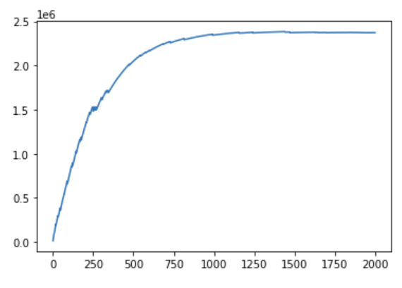
plt.plot(scores)
plt.show()
Output:

Most efficient path:
[26262, 1, 3, 6, 10, 16, 24, 36, 53, 79, 118, 176, 260, 382, 559, 817, 1195, 1751, 2569, 3772, 5536, 8120, 11902, 17438, 25546]
This code block outputs the actions corresponding to the node locations from the prior output, meaning the move to take at each hour of the day.
for step in steps:
    for state in state_lookup:
        if state_lookup[state] == step:
            print(state)
Output:

level1_(1,)
level2_(1, 1)
level3_(1, 1, 1)
level4_(1, 1, 1, 1)
level5_(1, 1, 1, 1, 1)
level6_(1, 1, 1, 1, 1, 1)
level7_(1, 1, 1, 1, 1, 1, 1)
level8_(1, 1, 1, 1, 1, 1, 1, 0
level9_(1, 1, 1, 1, 1, 1, 1, 0, 0)
level10_(1, 1, 1, 1, 1, 1, 1, 0, 0, 0)
level11_(1, 1, 1, 1, 1, 1, 1, 0, 0, 0, 0)
level12_(1, 1, 1, 1, 1, 1, 1, 0, 0, 0, 0, 0)
level13_(1, 1, 1, 1, 1, 1, 1, 0, 0, 0, 0, 0, 0)
level14_(1, 1, 1, 1, 1, 1, 1, 0, 0, 0, 0, 0, 0, 0)
level15_(1, 1, 1, 1, 1, 1, 1, 0, 0, 0, 0, 0, 0, 0, 0)
level16_(1, 1, 1, 1, 1, 1, 1, 0, 0, 0, 0, 0, 0, 0, 0, 0)
level17_(1, 1, 1, 1, 1, 1, 1, 0, 0, 0, 0, 0, 0, 0, 0, 0, 0)
level18_(1, 1, 1, 1, 1, 1, 1, 0, 0, 0, 0, 0, 0, 0, 0, 0, 0, 0)
level19_(1, 1, 1, 1, 1, 1, 1, 0, 0, 0, 0, 0, 0, 0, 0, 0, 0, 0, 1)
level20_(1, 1, 1, 1, 1, 1, 1, 0, 0, 0, 0, 0, 0, 0, 0, 0, 0, 0, 1, 1)
level21_(1, 1, 1, 1, 1, 1, 1, 0, 0, 0, 0, 0, 0, 0, 0, 0, 0, 0, 1, 1, 1)
level22_(1, 1, 1, 1, 1, 1, 1, 0, 0, 0, 0, 0, 0, 0, 0, 0, 0, 0, 1, 1, 1, 1)
level23_(1, 1, 1, 1, 1, 1, 1, 0, 0, 0, 0, 0, 0, 0, 0, 0, 0, 0, 1, 1, 1, 1, 1)
level24_(1, 1, 1, 1, 1, 1, 1, 0, 0, 0, 0, 0, 0, 0, 0, 0, 0, 0, 1, 1, 1, 1, 1, 1)
Notice we can compare the output of the brute force model to the reinforcement Q-learning model
Output:
brute force: {7622: (1, 1, 1, 1, 1, 1, 1, 0, 0, 0, 0, 0, 0, 0, 0, 0, 0, 0, 1, 1, 1, 1, 1, 1)}
Q-learning: level24_(1, 1, 1, 1, 1, 1, 1, 0, 0, 0, 0, 0, 0, 0, 0, 0, 0, 0, 1, 1, 1, 1, 1, 1)
While these outputs are the same, there is one key item to note: brute force takes 1 minute and 30 seconds, as compared to Q-learning which takes 240 microseconds. Which means that if a system needs to make decisions real-time, the only solution would be Q-learning. In conclusion, the simple model implies that it actually would be possible to create an AI control system that determines the operatiors action plan for a given period of time. The next goal would be to have the model run every 1 minute, with a 15 minute action plan provided. Also, receiving accurate forecasts from the solar systems likely production.