bmripper
Data Analytics
This project demonstrates my work in advanced business analytics, specially applying statistics and distribution models to business data. In this project, I show how one can use distribution models to “fill-in” data gaps due to only having collected limited data. In order to do this, we first determine a theoretical/appropriate data distribution using domain knowledge. For example, for filling in height data, one would assume a normal distribution. Another example, for counting the number of hurricanes in Florida, one would assume a Poisson distribution. Once we determine the theoretical model, we learn the parameters that minimize error, typically using Maximum Likelihood Estimating. We can then get a continuous data distribution which we can use to predict likely outcomes from unseen data.
| header | value |
|---|---|
| Author: | Ripperger, Brent |
| Date Created: | 28 November 2021 |
Hazard rate of divorce in the USA
In my example project, we look at USA divorce data. We are going to show the probability of a divorce over time from a sample of people, the years they’ve been married/divorced, and if they divorced. Your first thought might be, why are we using non-business data? For example purposes, this dataset is easy to explain and quick to grasp. The results are also intuitive. However, a business example for this exact same problem would be: predict when a piece of equipment will breakdown. Say we had a dataset of equipment IDs, the amount of time the equipment has been operational, and is it running or not. We are going to determine the hazard curve for this dataset (i.e., what is the probability a piece of equipment breaks down each year in operation). We are doing all these steps for divorce data as our example.
Metadata
| header | value |
|---|---|
| Title | Divorce data in USA |
| Dimensions | 3367 rows x 3 columns |
top 4 rows:
| ID | time between marriage and divorce or end of observation | divorce or not |
|---|---|---|
| 9 | 10 | No |
| 11 | 34 | No |
| 13 | 2 | Yes |
| 15 | 17 | Yes |
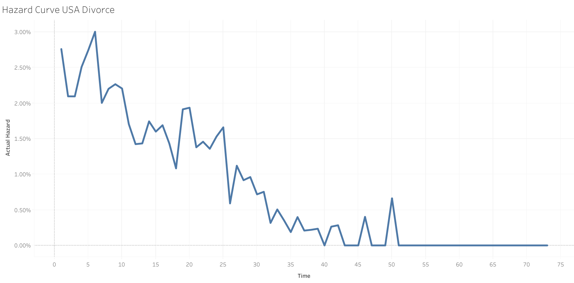
Aggregate Data
We need to compute the actual hazard rate at each year. Therefore, we aggregate the IDs into a countdown of remaining population at each year in the dataset (0-73 years).
top 4 rows:
| time | population at time t | actual hazard ratio |
|---|---|---|
| 1 | 3367 | 0.027621028 |
| 2 | 3147 | 0.020972355 |
| 3 | 3005 | 0.020965058 |
| 4 | 2869 | 0.025095852 |
Apply Distribution Model
We now will apply the 2-parameter Weibull distribution model. The Weibull model is great because it has only two parameters, but those two parameters allow it be very flexible and adapt to many data distributions. We will use maximum likelihood estimating to determine the optimal parameters (lambda and c) for this model. However, we are also going to make the underlying assumption that there are two “groups” of people in our dataset. Meaning, there isn’t just one “divorce rate” among all people. We are going to assume there are actually two groups with different divorce rates. Therefore, we will have four parameters (lambda1, c1, lambda2, c2).
| parameter | value |
|---|---|
| lambda1 | 0.0404 |
| c1 | 1.1887 |
| lambda2 | 0.0188 |
| c2 | 0.0010 |
| prop. group 1 | 0.4292 |
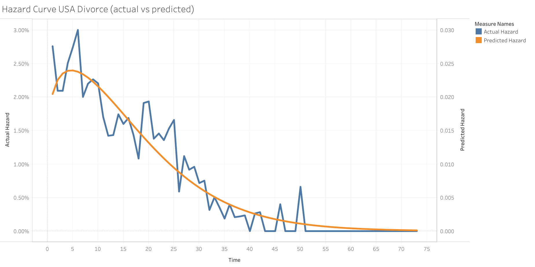
Interpretation
What is the final conclusion? From the limited data provided, we were able to produce a continuous curve that fits our dataset extremely well. For any point in time, whether it’s 4 years or 4.152 years, we have a quality estimate for the probability someone will get divorced. We also were able to determine that there are likely two groups within our dataset (~43% follow hazard ratio group 1, 57% follow hazard ratio group 2). We can see that in year 5, the highest probability of getting divorced occurs. However, each year after year 5, the odds of a divorce lessens. Notice how at year 50, there was a spike in the actual hazard ratio while our model stays consistent. That is due to the properties of our model choice. This is sometimes a very desirable result, and goes to show how using distribution models can extrapolate from limited data. If we relied solely on our dataset, our probability prediction would be too volatile at year 50. The Weibull model is actually more stable and intuitive. There are many distribution models to apply to various problems. The trick is to have someone that can choose the optimal distribution.